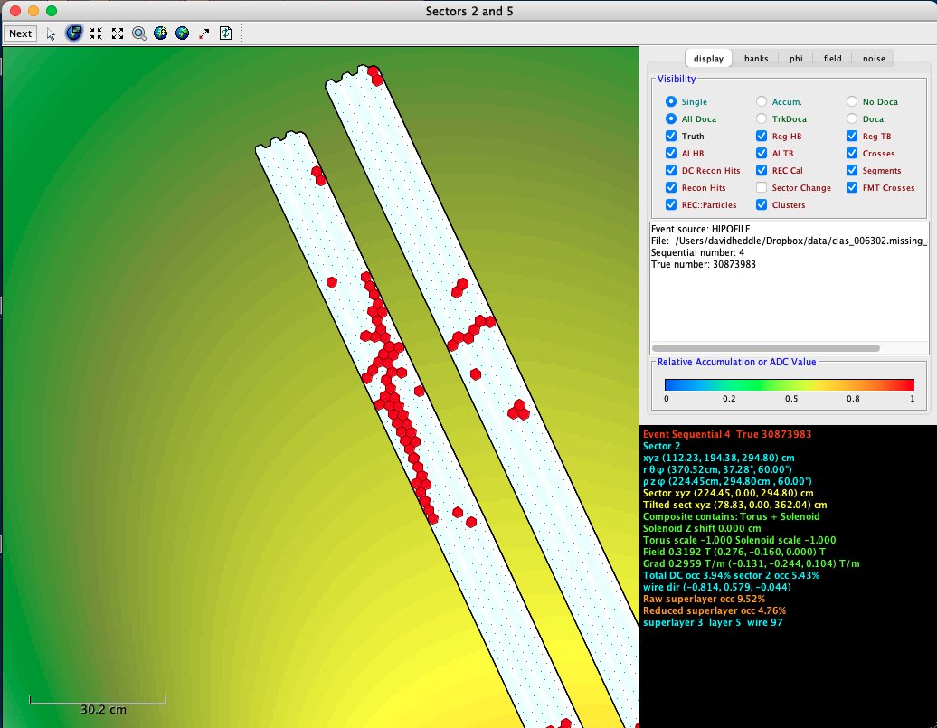
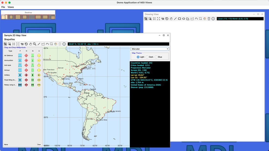
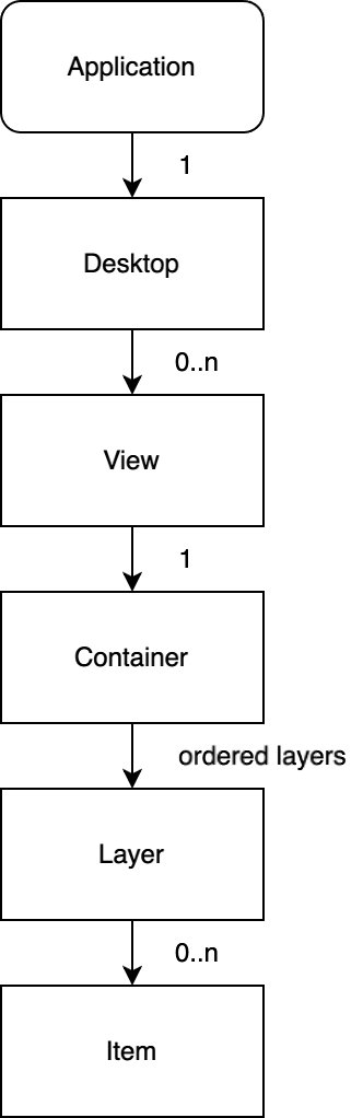
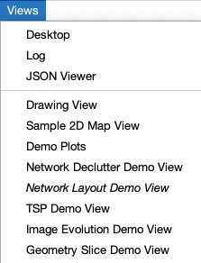
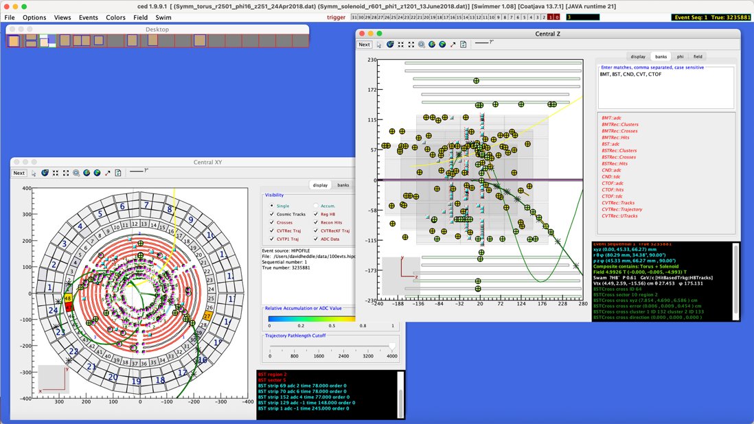
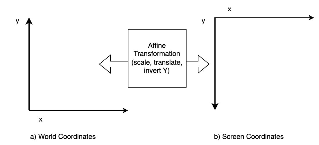
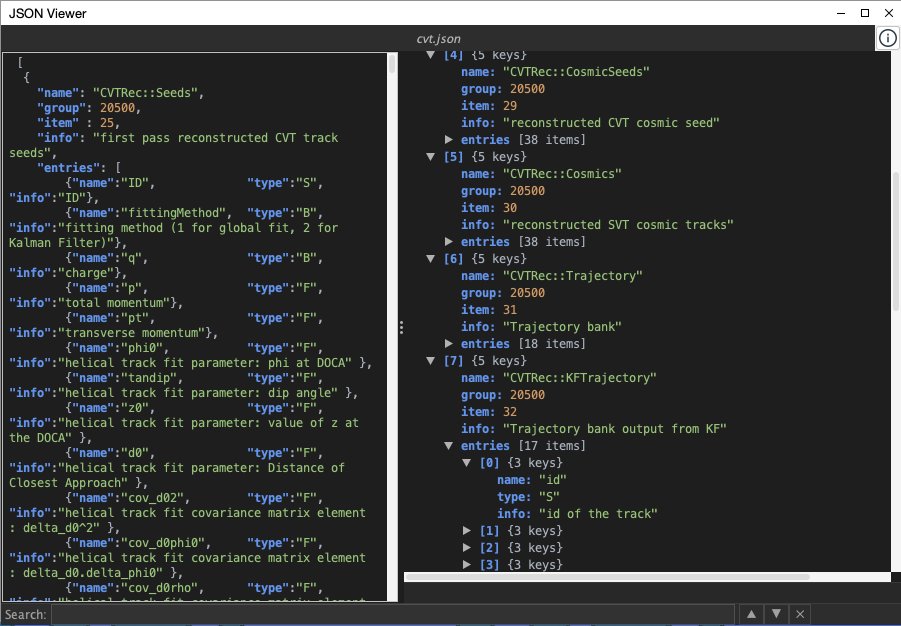
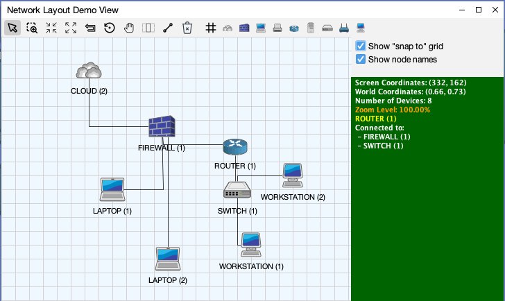
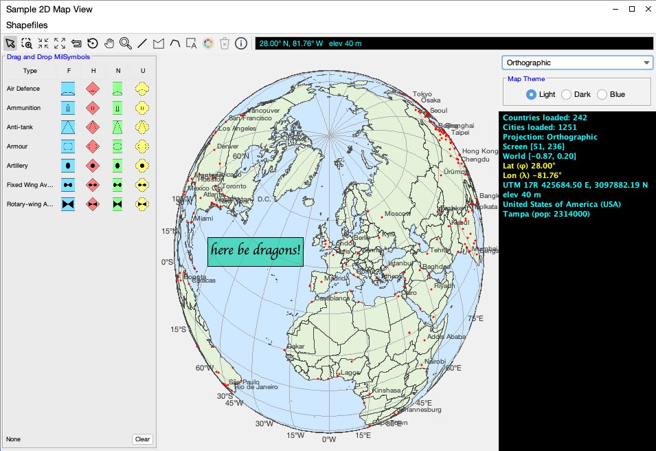
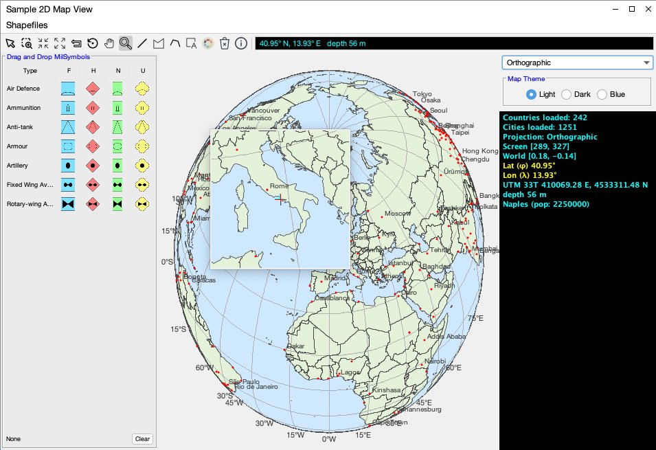
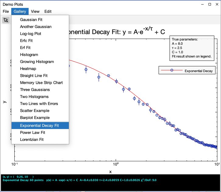
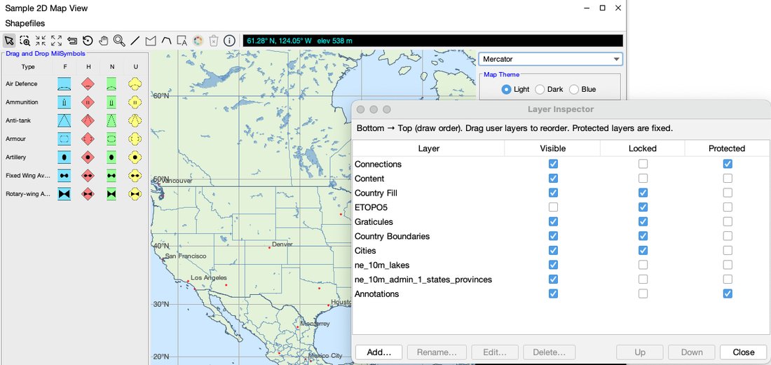
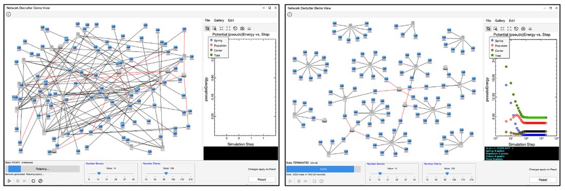
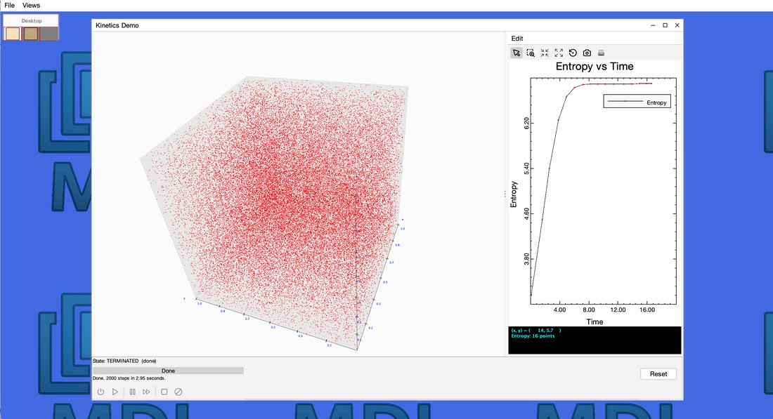
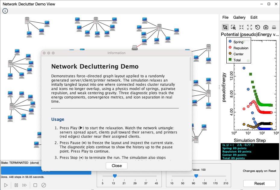
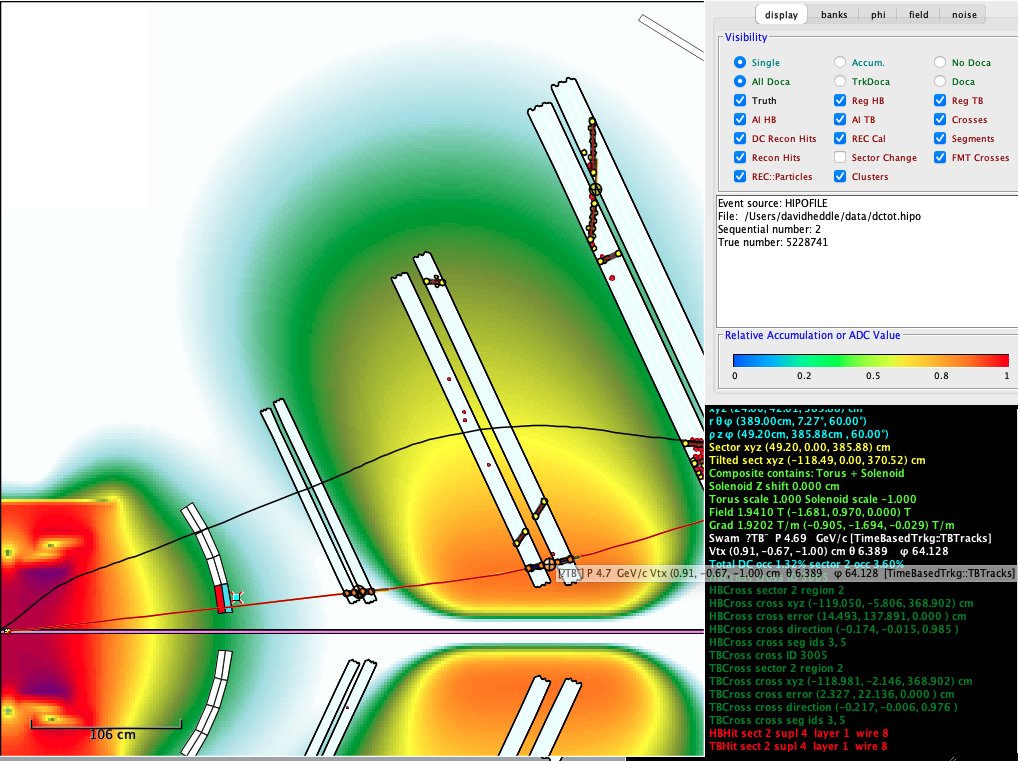
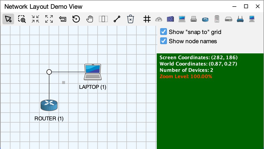
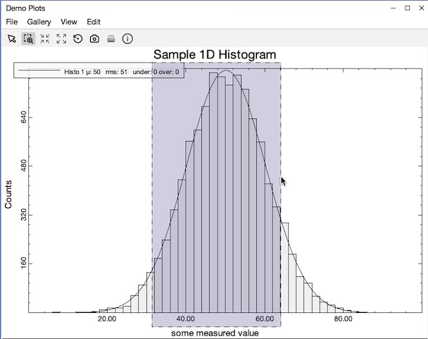
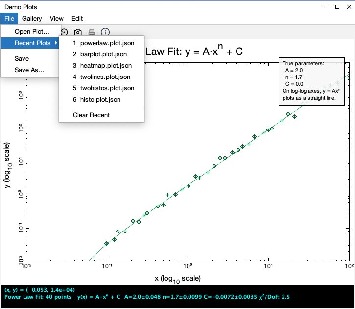
Figure 1-1. A MDI visualization of a nuclear physics detectorFigure 1-2. The MDI DemoApp as it appears at startupFigure 1-3. The MDI visual element hierarchyFigure 1-4. The Views menu for the MDI DemoAppFigure 1-5. The VirtualView enables point, click, and drag navigation of the VirtualDesktopFigure 1-6. Two independent views showing different representations of the same dataFigure 1-7. The container handles the transformation from world to screen coordinatesFigure 1-8. The JsonView is an example of a containerless "administrative" viewFigure 1-9. The Network Layout Demo View from the MDI DemoApp has connections on the Connections Layer and network components (items) placed in the Content layerFigure 1-10. A text annotation drawn onto the MapView from the MDI DemoAppFigure 1-11. The toolbar for the Map2D view was configured with a Magnify tool, which most toolbars will omitFigure 1-12. The Demo Plots view showing the result of an exponential decay fit with a logarithmic x-axisFigure 1-13. The DemoMap combines GeoJSON and ESRI shapefile data, with each geographic component managed as an MDI layer and appearing in the Layer InspectorFigure 1-14. The starting and ending visualizations in the Network Declutter Demo ViewFigure 1-15. The completion of a simulation in a 3D view, modeling the free expansion of an ideal gas
Chapter 2 — Creating the Application
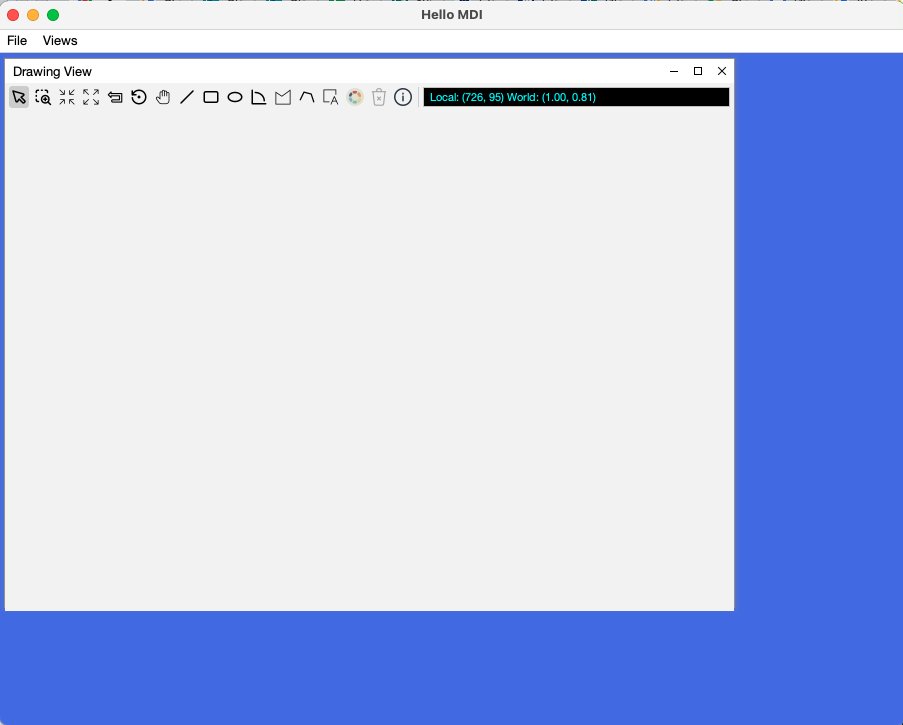
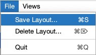
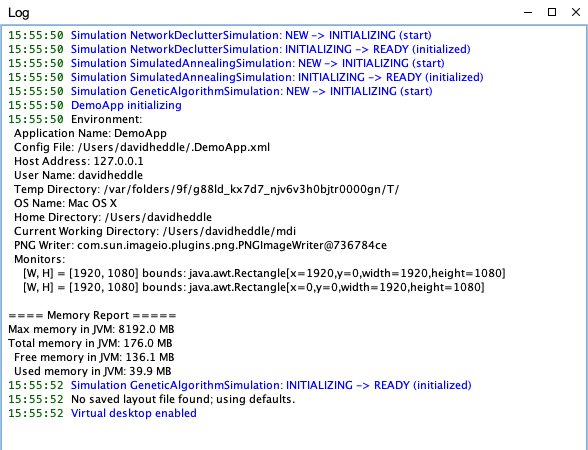
Figure 2-1. The HelloMDI application at startupFigure 2-2. The File menu is used to manage layout persistenceFigure 2-3. A self-dismissing toast notifies the user that a saved layout has been appliedFigure 2-4. A LogView for the MDI DemoApp just after startup. Messages are color-coded by severity within the LogPane
Chapter 3 — Creating Views
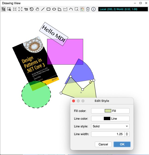
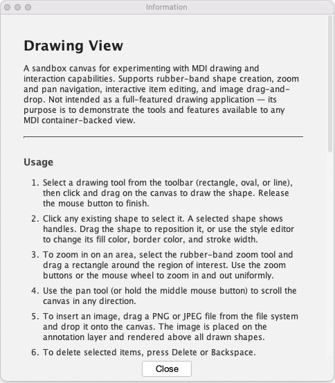
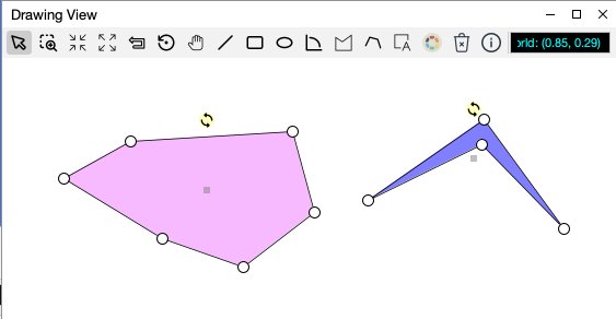
Figure 3-1. A portion (there's more, hence the scrollbar) of the ViewInfo for the NetworkDeclutterDemoViewFigure 3-2. The DrawingView with the style editorFigure 3-3. The custom ViewInfo created for the DrawingViewFigure 3-4. An example of feedback and hoveringFigure 3-5. A complex administrative view
Chapter 4 — Items
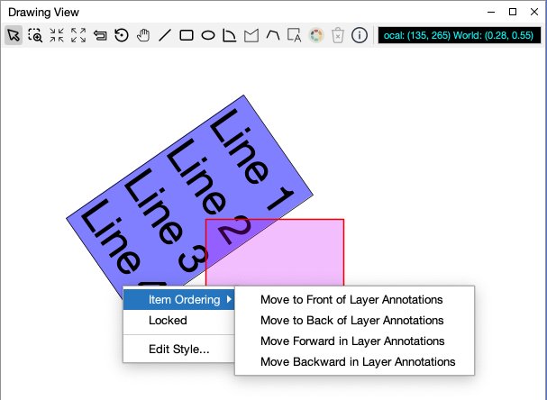
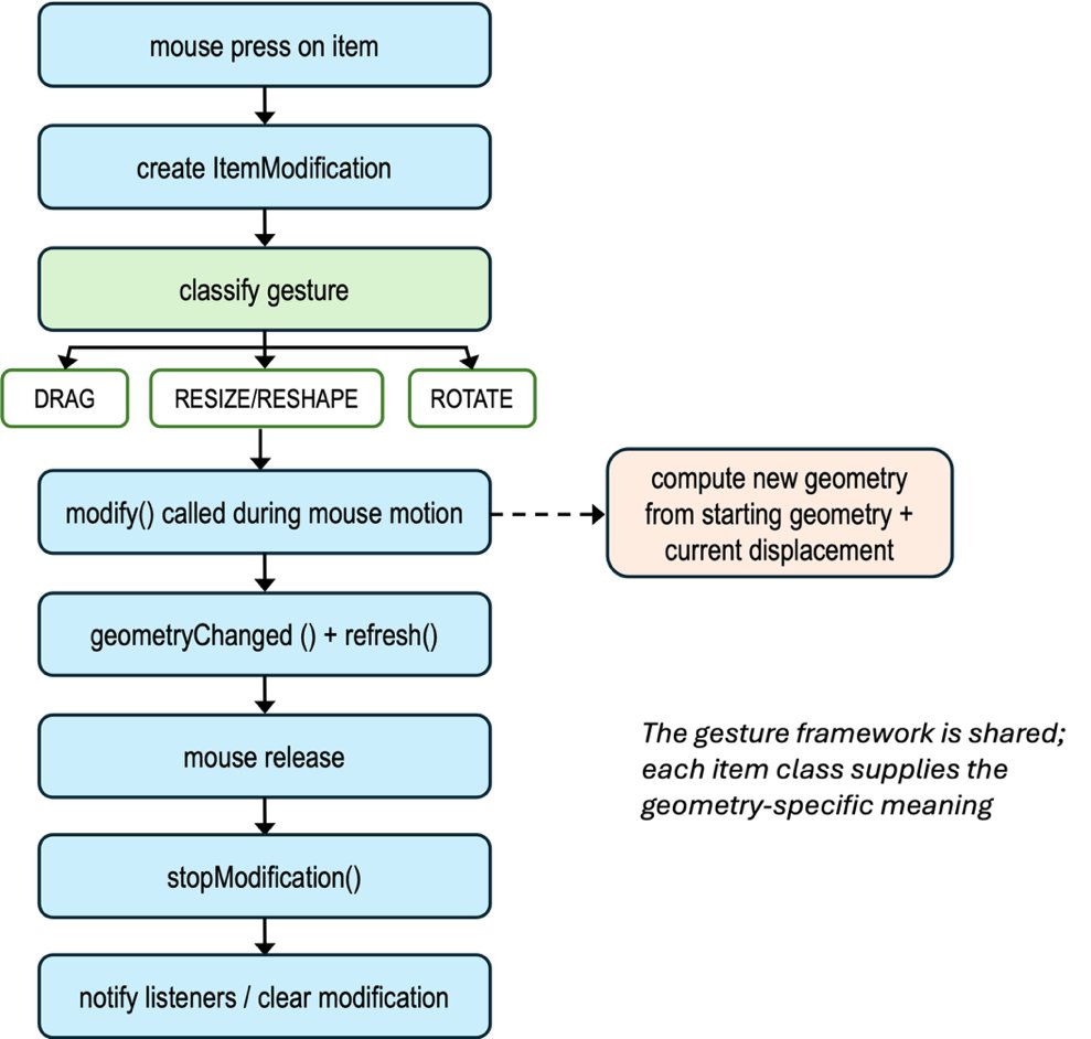
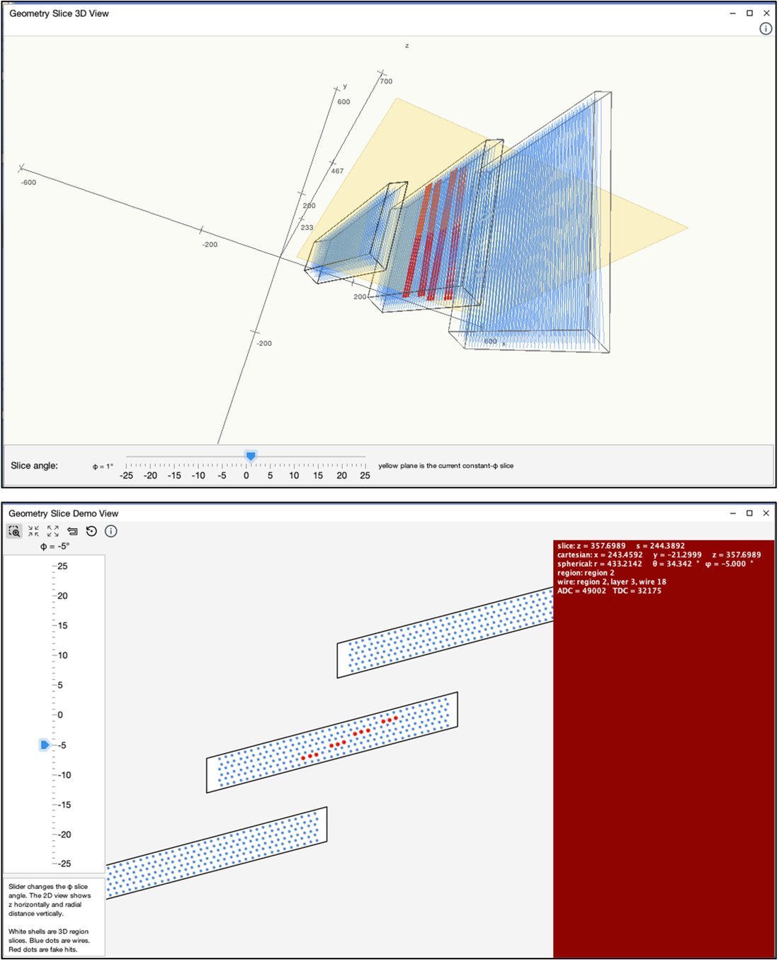
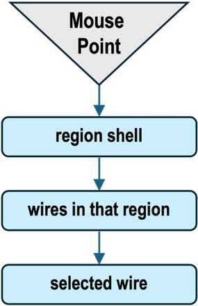
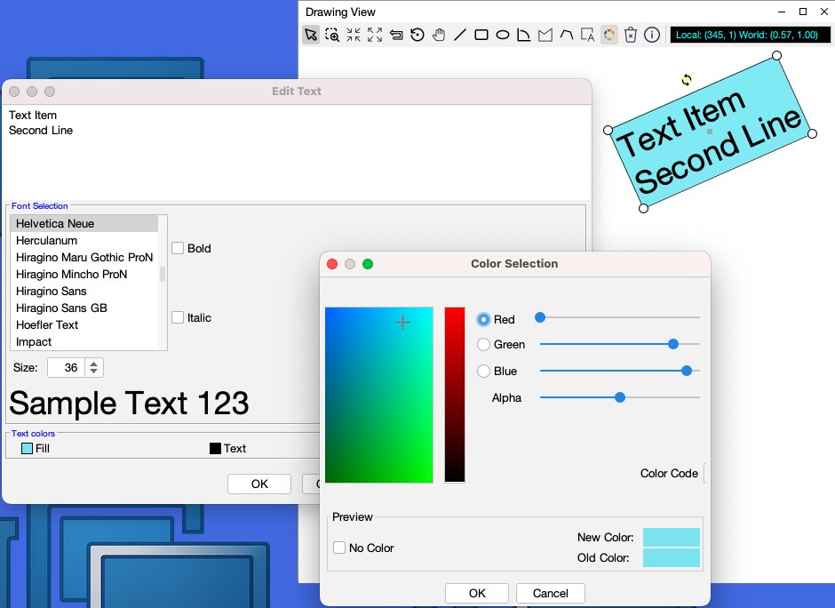
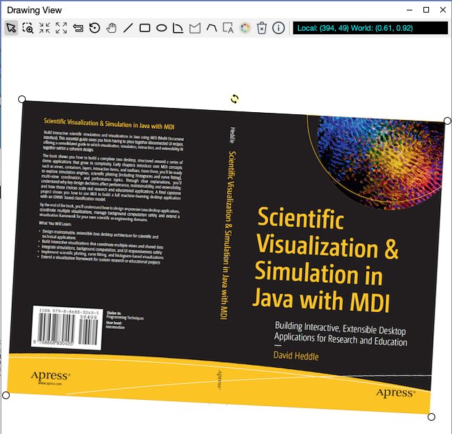
Figure 4-1. Combining direct drawing (magnetic field and tracks) with item drawing (detector components)Figure 4-2. When an item is selected, its focus is drawn as a small gray squareFigure 4-3. The item popup menu gives the user z-order controls within the item’s layerFigure 4-4. The item-modification lifecycle, from mouse press through gesture classification, repeated modify() calls, and final notificationFigure 4-5. The top view shows the 3D geometry, including region shells, wires, hit wires, and the current constant-φ slice plane, while the lower view shows the corresponding 2D slice through the same modelFigure 4-6. Staged hit testing narrows the search from a region shell to the wires within that regionFigure 4-7. A TextItem combines editable text, font selection, color styling, and ordinary item handlesFigure 4-8. An ImageItem displays a raster image while remaining a fully interactive item, complete with selection, resizing, and rotation handlesFigure 4-9. A selected ConnectorItem links two items and exposes its editable elbow
Chapter 5 — Toolbars and Rubberbanding
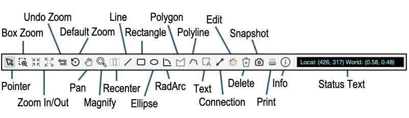
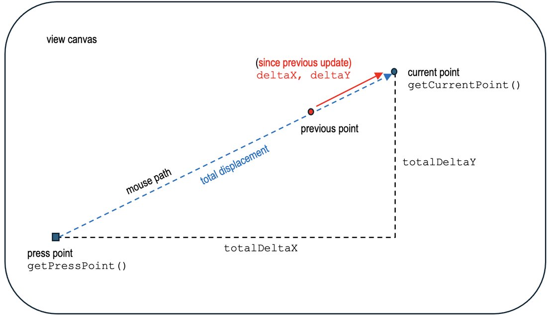
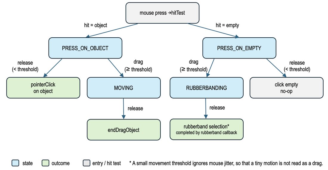
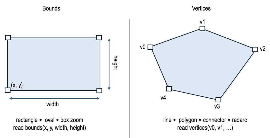
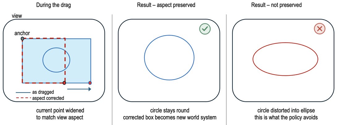
Figure 5-1. A standard MDI toolbar assembled from ToolBits, with the predefined tool buttons labeledFigure 5-2. A GestureContext carries both incremental and total displacement; the operation decides which to useFigure 5-3. The pointer tool's internal state machine, driven by press, threshold crossing, and releaseFigure 5-4. A rectangle-based tool reads bounds; line and polygon tools read collected verticesFigure 5-5. Box zoom with the RECTANGLE_PRESERVE_ASPECT policy adjusts the dragged rectangle to the view's aspect ratio, so the new world system is not distortedFigure 5-6. Histograms are an example where the XONLY rubberband policy is usefulFigure 5-7. Drawn toggle buttons used as small animated controls; the icon graphics are generated by Java code rather than image resourcesFigure 5-8. The map view’s status text provides a quick reference to the latitude, longitude, and elevation at the current mouse location
Chapter 6 — Plotting (sPlot)
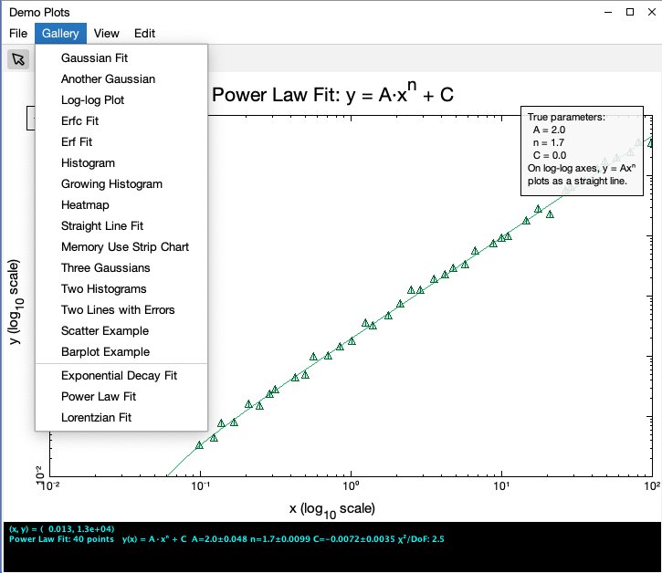
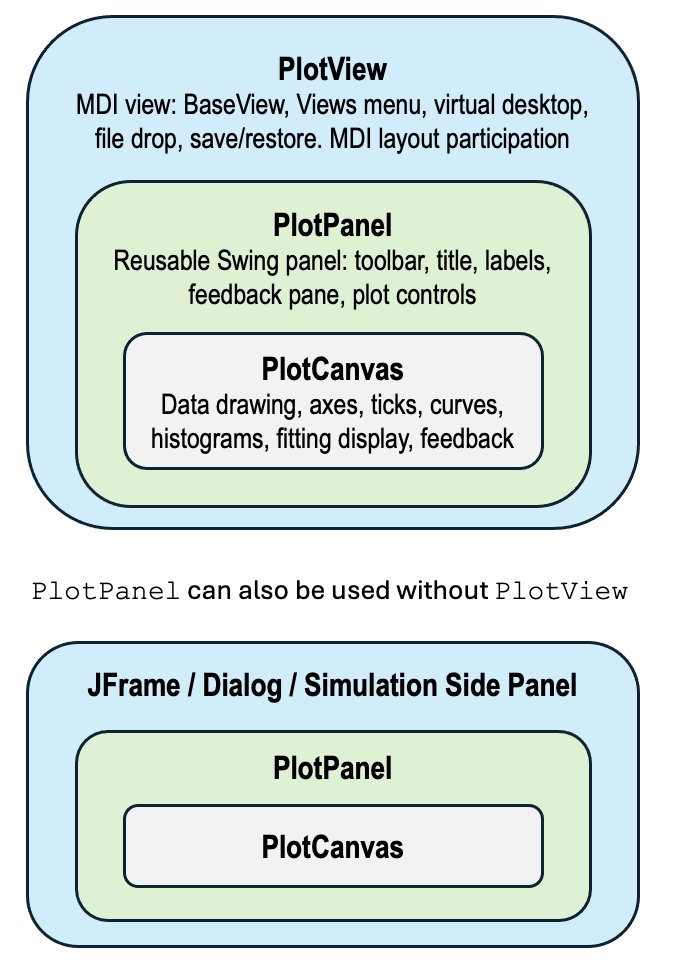
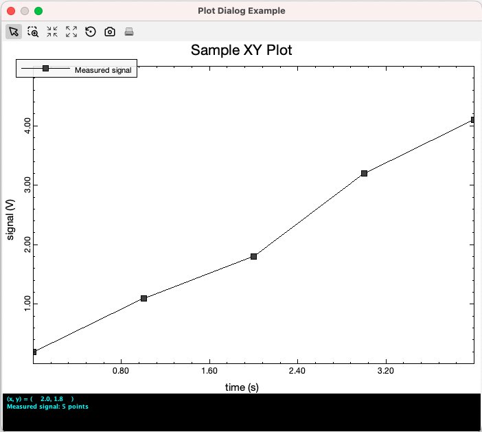
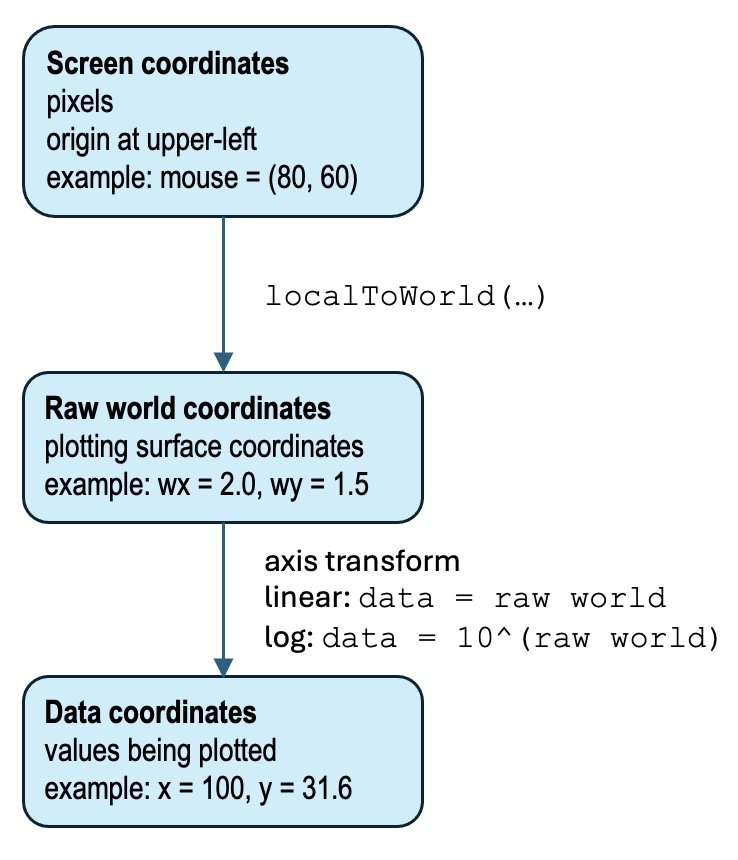
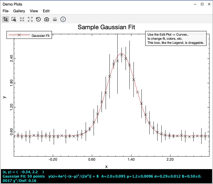
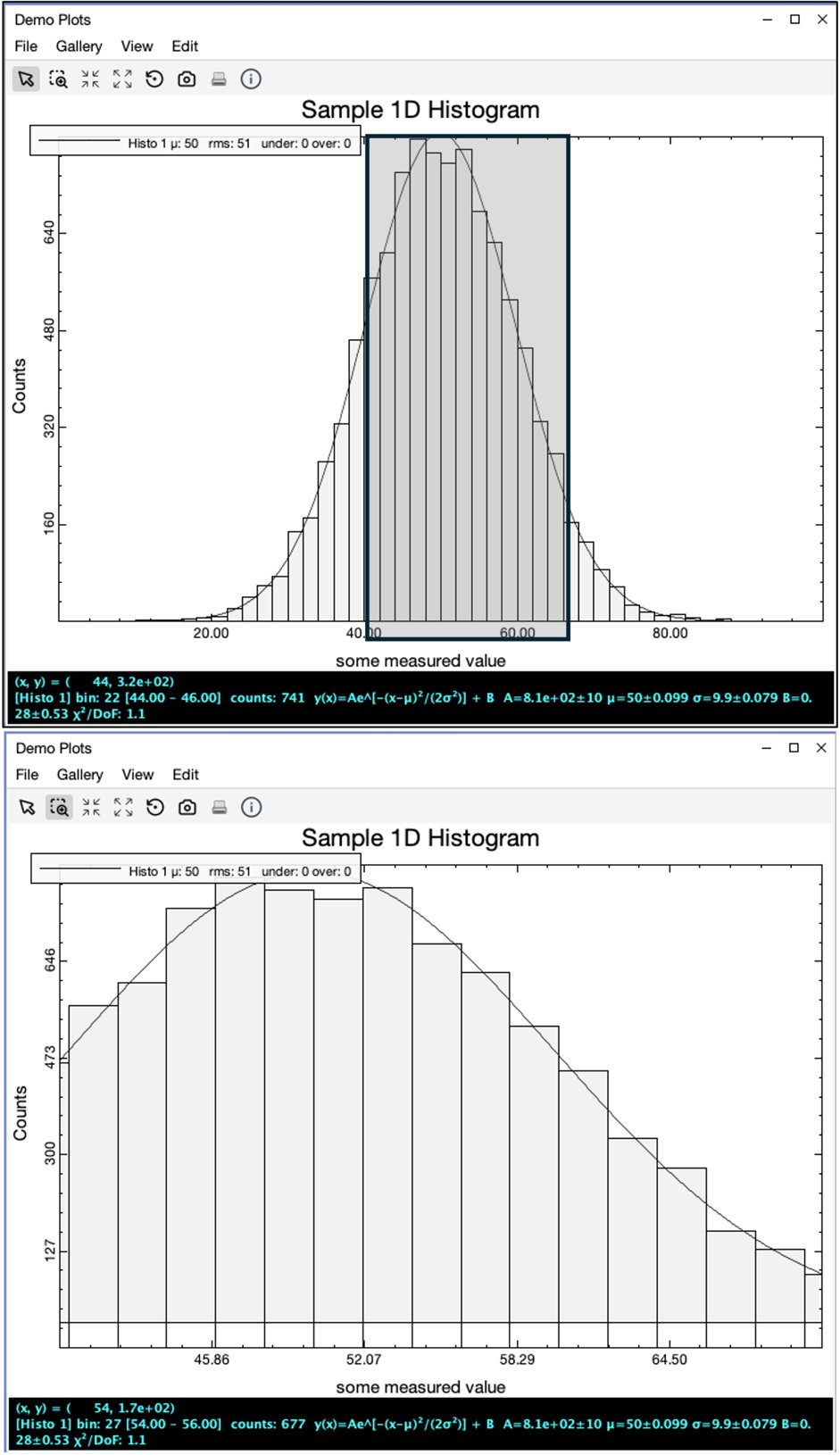
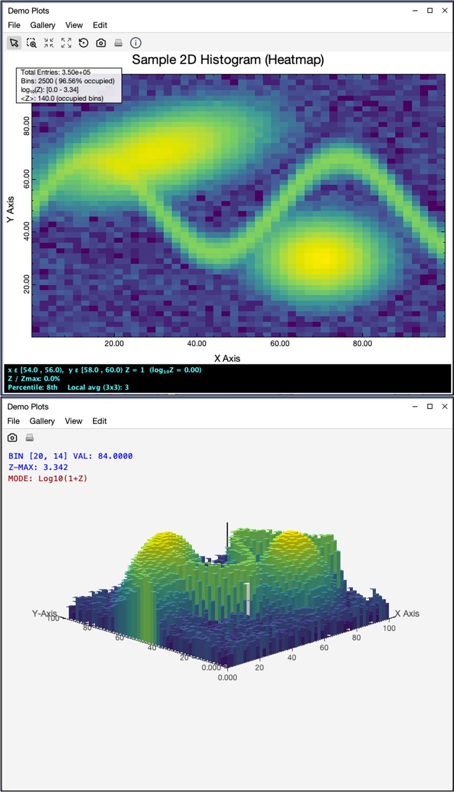
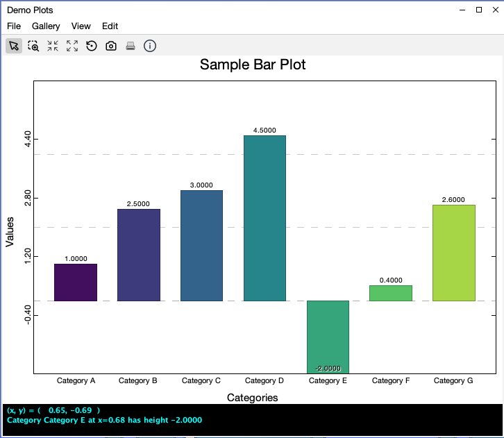
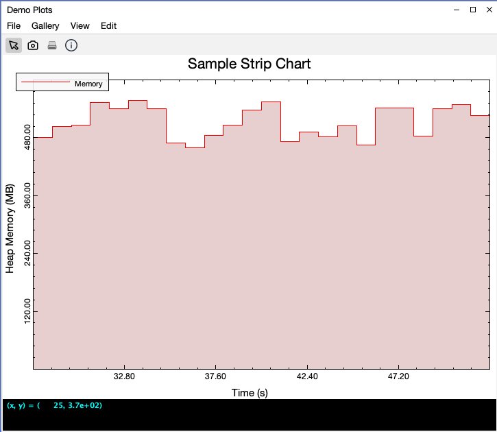
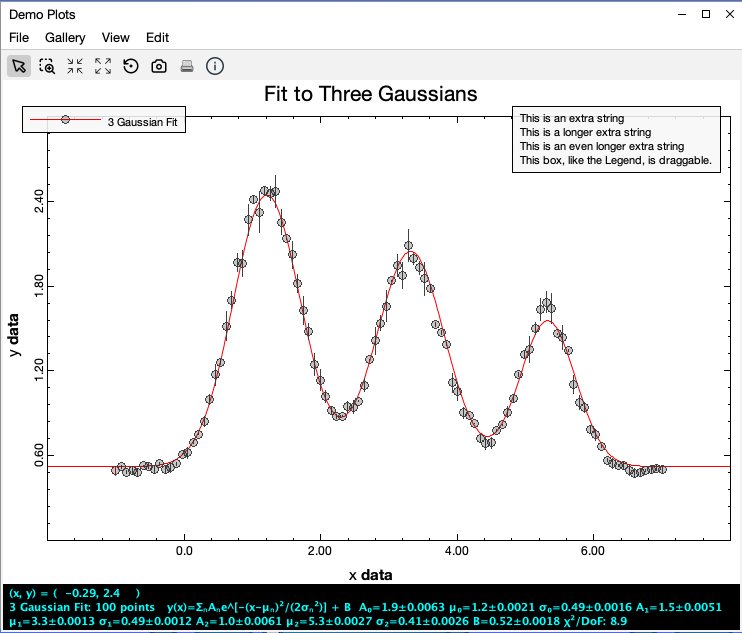
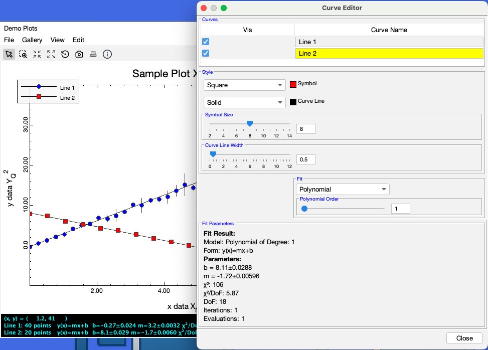
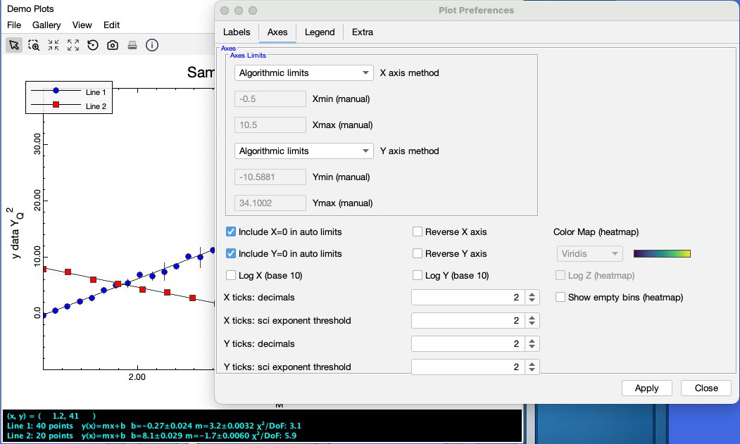
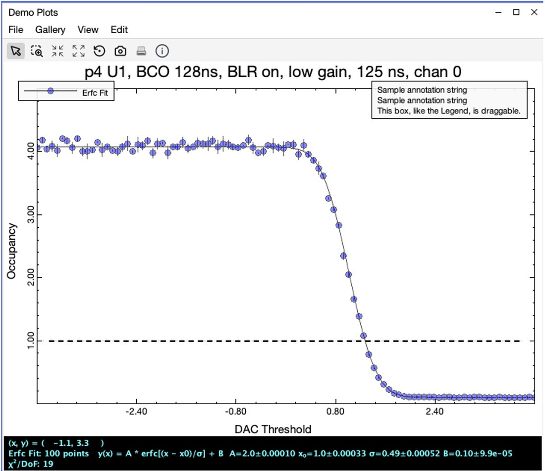
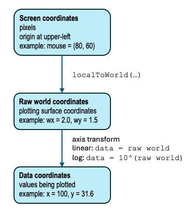
Figure 6-1. The Demo Plots view in the MDI DemoApp, showing a plot hosted as a normal MDI view and a gallery of sample plotsFigure 6-2. A PlotView hosts a PlotPanel, and the PlotPanel decorates a PlotCanvas that owns the plot data and rendering stateFigure 6-3. A minimal XY plot consisting of PlotData, one Curve, a PlotCanvas, and a PlotPanel displayed in a JDialogFigure 6-4. PlotCanvas translates among screen coordinates, raw world coordinates, and data coordinatesFigure 6-5. The plot feedback pane reports mouse position and data-specific information without cluttering the plot areaFigure 6-6. A histogram uses an XONLY box-zoom policy (top) and the resulting zoomed plot (bottom)Figure 6-7. A 2D histogram displayed in Standard Plot heatmap mode with mouse feedback (top) and pseudo-3D Histogram mode (bottom)Figure 6-8. A simple bar plotFigure 6-9. A constantly updating memory usage strip chartFigure 6-10. A three-Gaussian fit to data with error barsFigure 6-11. The curve editor for a plot with two curvesFigure 6-12. The same two-curve plot along with one tab from the preferences editorFigure 6-13. A plot with an added reference line and some extra textFigure 6-14. The File menu on a PlotView provides support for saving and loading plots
Chapter 7 — Mapping
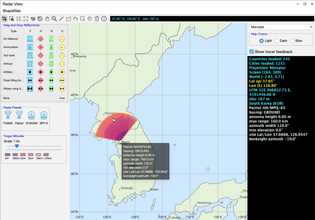
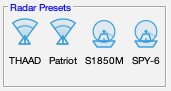
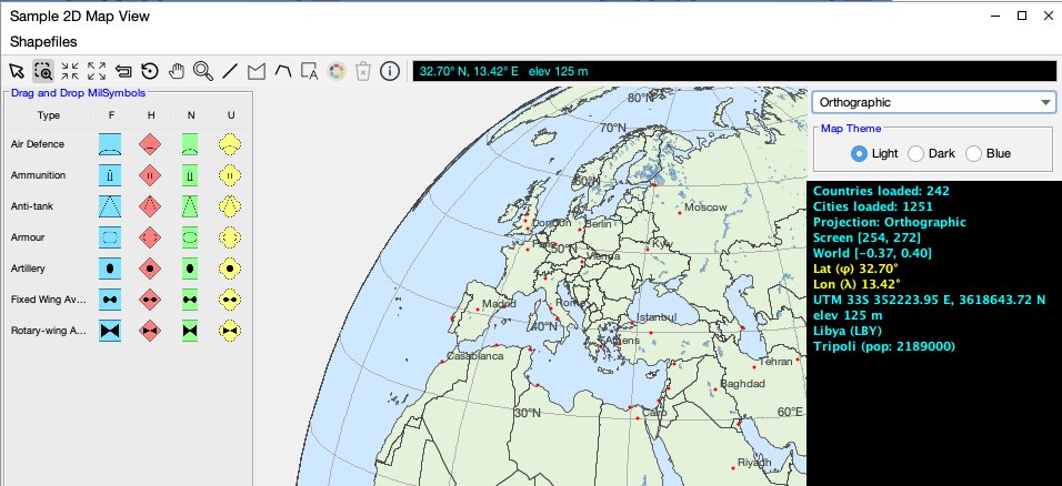
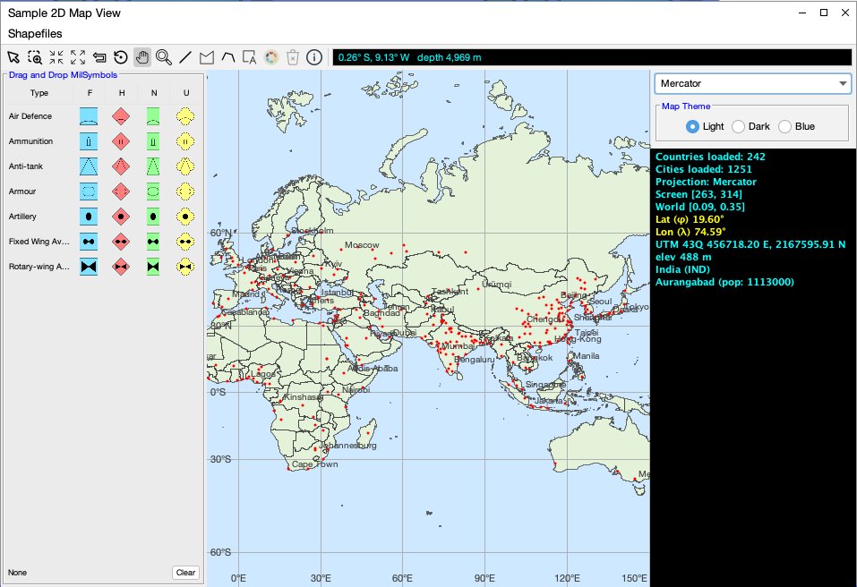
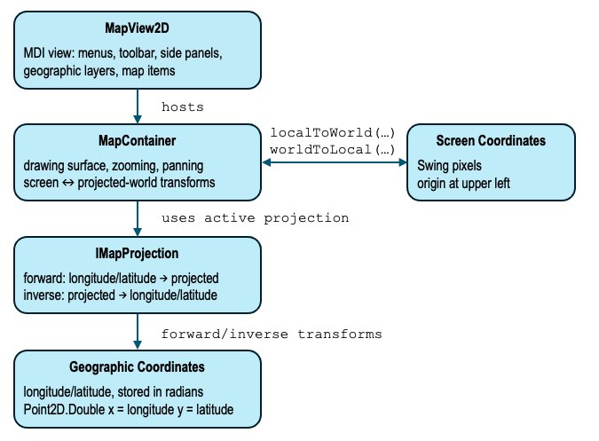
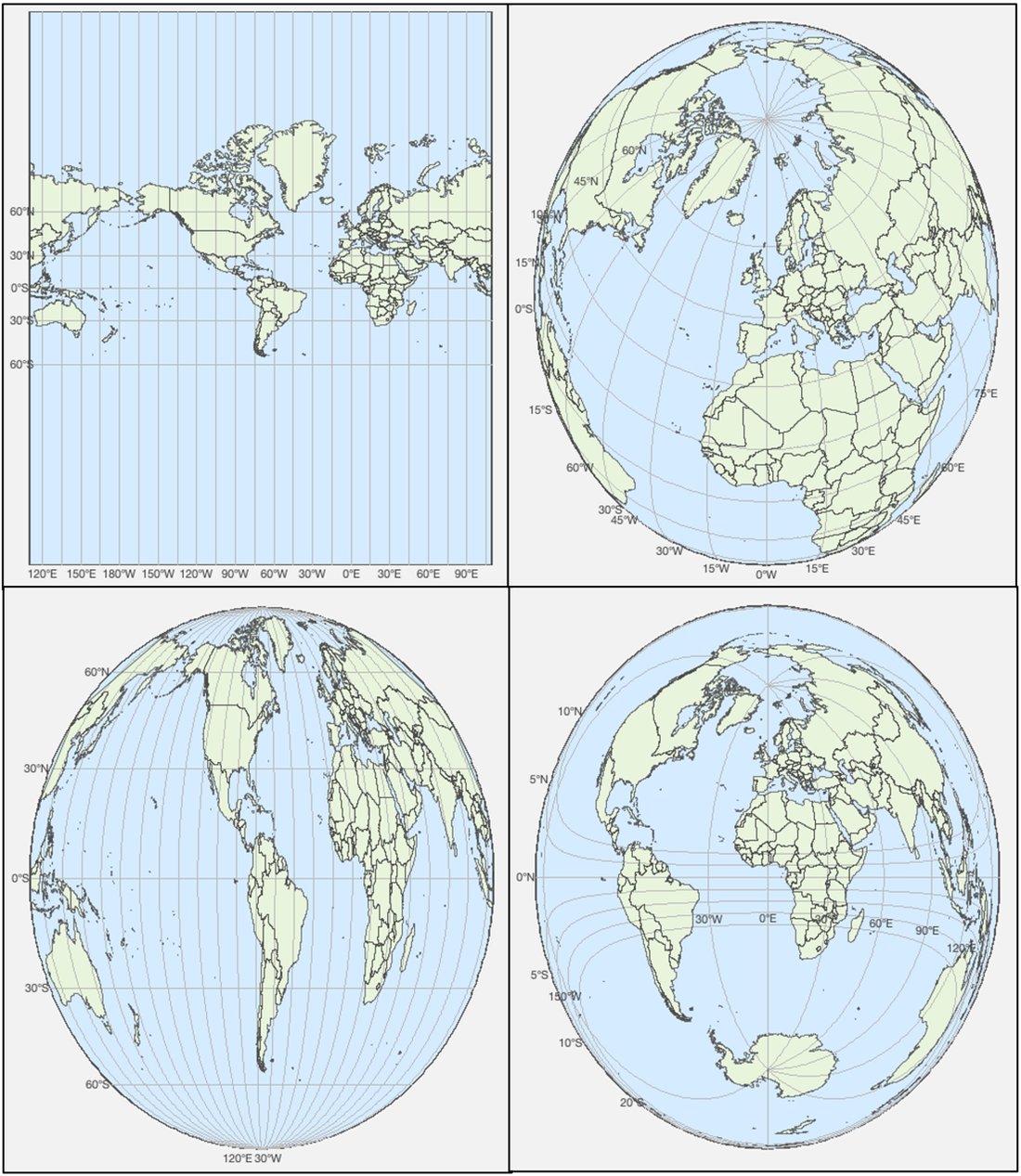
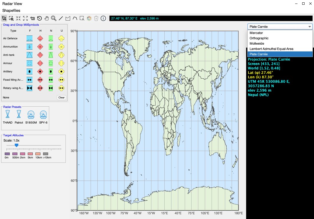
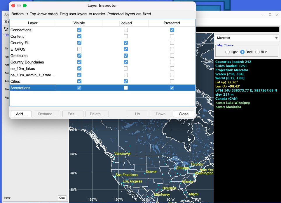
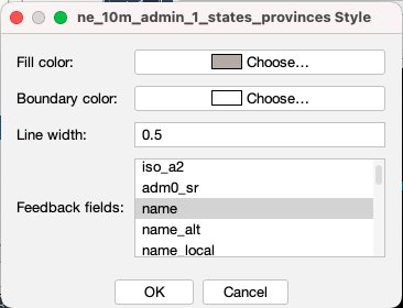
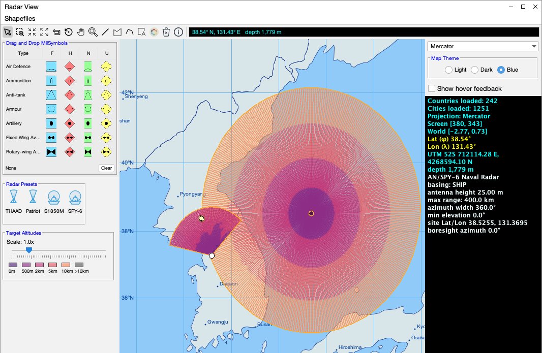
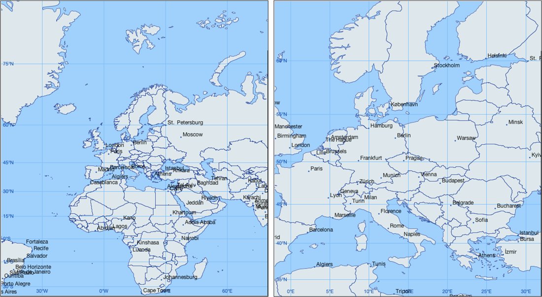
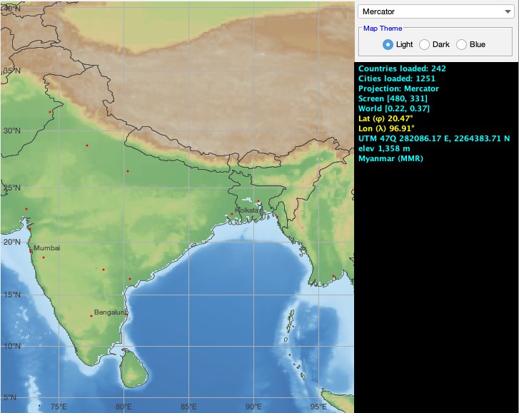
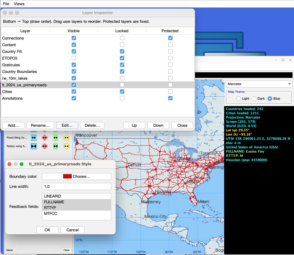
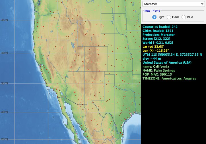
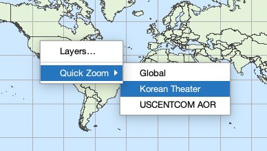
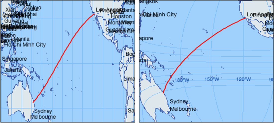
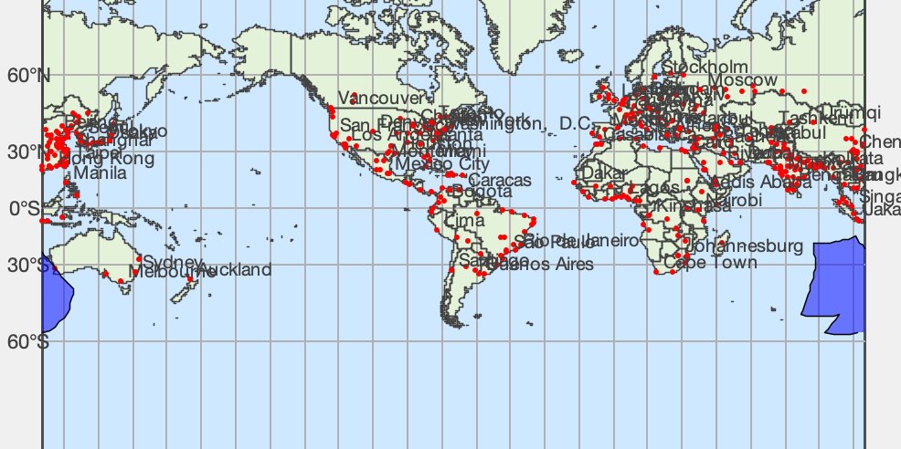
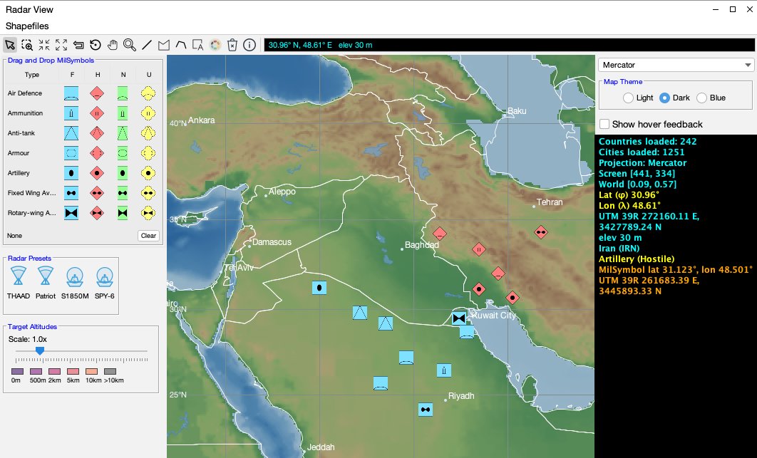
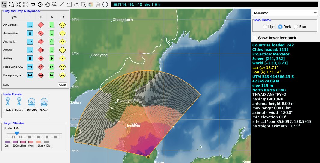
Figure 7-1. The Sample 2D Map View in the MDI DemoApp, with the compact projection-and-theme control panel, NATO symbol picker, feedback pane, and map toolsFigure 7-2. MapView2D hosts a MapContainer and an active IMapProjection; specialized map layers supply the geographic context, while map-item layers supply interactive application objectsFigure 7-3. Map coordinate conversion proceeds from screen coordinates to projected world coordinates and then through the inverse projection to longitude and latitudeFigure 7-4. The four built-in projections at full extent: Mercator (top-left), Orthographic (top-right), Mollweide (bottom-left), and Lambert Azimuthal Equal-Area (bottom-right)Figure 7-5. The application-supplied Plate Carrée projection appears in the radar application’s projection selector alongside the four built-in projectionsFigure 7-6. The map layer stack shown in the Layer Inspector, with two added shapefiles for lakes and statesFigure 7-7. The capability-driven layer-style editor configured for a polygon shapefile layerFigure 7-8. The radar application adds a hover-feedback checkbox to the standard MapControlPanel, while radar presets, NATO symbols, and target-altitude controls remain in the domain-specific side panelFigure 7-9. Adaptive graticules at two zoom levels, showing denser coordinate spacing after zooming into a smaller regionFigure 7-10. ETOPO5 elevation and bathymetry rendered through the active projection, with country boundaries remaining crisp above the terrainFigure 7-11. A nationwide primary-roads shapefile displayed as an MDI layer. The layer editor selects DBF attributes for pointer feedback, while the Layer Inspector controls visibility and drawing orderFigure 7-12. The feedback pane reporting projection, screen and world coordinates, longitude, latitude, UTM coordinates, elevation or depth, and picked geographic featuresFigure 7-13. The quick zoom feature gives the user the ability to quickly move to a region of interestFigure 7-14. The same great-circle route in two projections, demonstrating that one geographic path can have different projected shapesFigure 7-15. A geographic polygon crossing a projection seam, rendered as safe projected subpaths rather than as an erroneous line through the mapFigure 7-16. NATO military symbols placed as geographic MDI items using the icon picker beside the demonstration mapFigure 7-17. A selected sector radar item showing its geographic line-of-sight coverage fan
Chapter 8 — Simulation
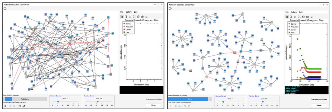
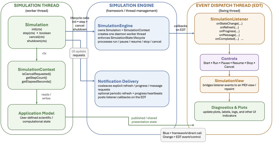
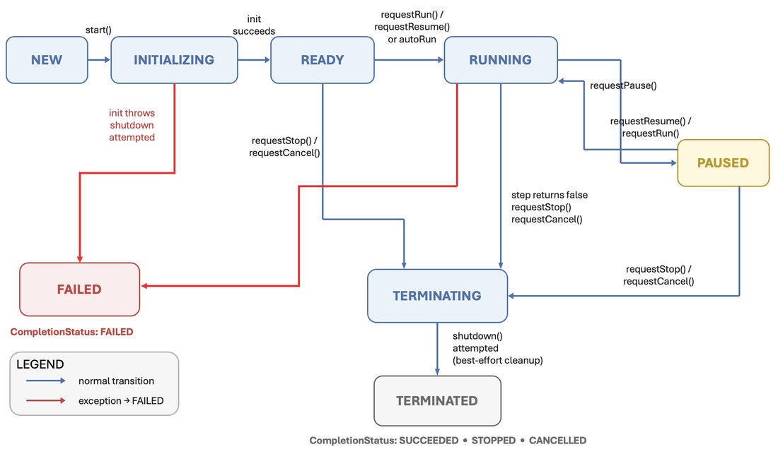
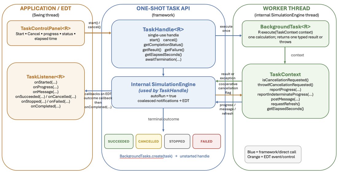
Figure 8-1. The network-decluttering simulation before relaxation (left) and after the force-directed layout has converged (right)Figure 8-2. The simulation architecture separates the computation and its context from the MDI view, controls, diagnostics, and other Swing componentsFigure 8-3. The SimulationEngine lifecycle, including initialization, ready, running, paused, terminating, terminated, and failed statesFigure 8-4. A one-shot task performs one calculation on a worker thread and delivers progress and terminal callbacks on Swing’s EDTFigure 8-5. The custom network control panel combines the standard simulation controls with sliders that define the next randomized model
 MDI Companion